
The Matlab script Examples/LongRangeZerothOrder.m() examplifies the typical workflow of the synapse generation pipeline.
Before running it, make sure that your Matlab path points to the synGenPipeline folders, by running pathme.m().
The main steps of LongRangeZerothOrder are:
Implemented is a very crude model of Thalamocortical projections on L4 pyramidal neurons. Pyramidal dendrite densities are given by two Gaussians, rotation symmetric around the vertical axis:
Together their shape can second best be described as a lava lamp. Thalamocortical axon arborizations are modelled as quasi-randomly placed spherical Gaussians. The pyramidal densities are placed upright in the neuropil, with the orientation of their apical dendrites perturbed by an angle normally distributed around zero with a standard deviation of 0.15 rad.
clear variables
% if not already done: add synGenPipeline functions to the Matlab path
run(['..' filesep 'pathme'])
%number of dimensions
lpar.nDim = 3;
%cutoff [number of sigma's] for generating target distribution
lpar.nSigRange = 3 ;

%voxel size and number
lpar.vox.voxelSize = 1;
lpar.vox.voxPerDim = 150 ;

%Defining the first post-synaptic neural population (lpar)
%Seed for this population
postPop.seed = 27552 ;
%Identification name
postPop.name = 'Pyramidal cells' ;
%Identification number
postPop.nr = 1 ;
%whether or not this is a presynaptic population
postPop.isPre = 0 ;

%Number of neurons in this population
postPop.Nn = 20 ;
%Where these soma exist, in normalized coordinates
postPop.soma.area = [.2 .8;.2 .8;.1 .7];
%soma distribution function
postPop.soma.distr = 'rand' ; %'qrand' 'unifRand' ,'unif' ||(debug: 'cen' 'diag')
%Seed for the distribution of the soma
postPop.soma.seed = 2421 ;

%anonymous function to the blob
postPop.typeSpec.generator = @(x) genPyr0(x); %See 'help blobs'
%paramters for the generator
postPop.typeSpec.tsz = 20 ;
postPop.typeSpec.tsr = 0.4;
postPop.typeSpec.bsxyr = 25;
postPop.typeSpec.bsr = 0.15 ;
postPop.typeSpec.dr = 1.55  ;
postPop.typeSpec.f =  0.3 ;
postPop.typeSpec.wVec = [0.5,1.5] ;

%Rotation angles, perturb around the vertical axis is a random direction
%Rotations are applied in the order x, y, then z.
postPop.rot.X = 0 ;
postPop.rot.Y = [0,0.15] ;
postPop.rot.Z = [0,pi] ;

%rotation distribution See 'help randSample'
postPop.rot.YDistr = 'normRand' ;
postPop.rot.ZDistr = 'unifRand' ;

%Trees balancing factor. See 'help MST_tree'
postPop.mst.bf = 0.55 ;
%Trees max branch threshold
postPop.mst.thr = 100 ;

%Assign postPop to the neurPop
lpar.neurPop{1} = postPop ;

%Define the second population (lpar)
prePop.isPre = true ;
prePop.Nn = 30 ;
prePop.seed = 18713 ;
prePop.name = 'Thalamocortical axons' ; %Identifier
%To specify the area where soma reside, you can also define the size of
%the edge where there are no soma. This is, like area, in normalized
%coordinates, so edge [0,0,5) ;
prePop.soma.edge = 0.1 ;

prePop.soma.distr = 'qrand' ; %'qrand' 'unifRand' ,'unif' ||(debug: 'cen' 'diag')
prePop.soma.seed = 294312;

prePop.typeSpec.generator = @(x) genGauss(x); %See 'help blobs'
%parameter for this generator
prePop.typeSpec.sig = [25 35] ;
prePop.typeSpec.sigDistr = 'unifRand' ;

%Trees balancing factor. See 'help MST_tree'
prePop.mst.bf = [0.4 0.6 ] ;
%Because there is no definition of bfDistr, unifRand will be used by default

%Trees max branch threshold.See 'help MST_tree'
prePop.mst.thr = 1000 ;

%assign
lpar.neurPop{2} = prePop ;
%First step, fixing lpar (e.g. translating soma.edge to soma.area) and
%sampling all stuff for Yinfo
disp('Preparation') ;
[lpar,Yinfo] = prepareForYgen(lpar) ;

%Generates the target density
disp('Generating target densities') ;
[Ypre,Ypost] = generateY(lpar,Yinfo) ;
The synaptic element generator (Y->X) that is used here is genRand1. This method needs a specified number of synaptic elements, an aimed in-population standard deviation. The method is able to remove overlapping synaptic elements. The following variables are used as inputs to the function genRand1
nSynPreMean = 3000 ;
nSynPreSig = sqrt(3000) ;
nSynPostMean = 300;
nSynPostSig = 40 ;
removeOverlap = true ;

disp('Generating presynaptic elements') ;
[Xpre] = genRand1(Ypre,nSynPreMean,nSynPreSig,removeOverlap) ;
disp('Generating postsynaptic elements') ;
[Xpost] = genRand1(Ypost,nSynPostMean,nSynPostSig,removeOverlap) ;
The TreeJitterAmplitude is used in growTrees. The generated synaptic elements are placed somewhere in the near the center of their voxel, normally distributed in 3 dimensions independently, with a standard deviation given by the TreeJitterAmplitude. Grow trees is a gateway function to the trees toolbox’ MST_tree. It generates branches between the generated synaptic elements in X by creating a weighted minimum spanning tree. The output if this function is a cell array of trees, and list which associates a branch order with each synaptic element.
disp('Generating presynaptic trees') ;
TreeJitterAmplitude = 0.3 ;
[ TreesPre,synBOpre ] = growTrees(lpar,Xpre,Yinfo,true,TreeJitterAmplitude*4) ;
disp('Generating postsynaptic trees') ;
[ TreesPost,synBOpost ] = growTrees(lpar,Xpost,Yinfo,false,TreeJitterAmplitude) ;
A connectivity matrix is generated from two sets of synatic elements. Everywhere where a presynaptic and a postsynaptic element occur in a voxel, a synapse is formed. The function returns a connectivity matrix a cell matrix containing the voxel numbers of the synapses between two neurons
disp('Generating Connectivity matrix') ;
[conMat,synNeurMap] = generateConnectivity(Xpre,Xpost) ;
disp('Calculating and showing measures') ;

Ymsrs = Ymeasures(Ypre,Ypost)
XmsrsPre = Xmeasures(lpar,Xpre)
XmsrsPost = Xmeasures(lpar,Xpost) ;
nBins = 10 ;
CMmsrs = conMatMeasures(conMat,nBins,false);
Associates branch orders to synapses by comparing the synaptic element branch order association in the synBO variable, to the the neuron-synapse association in the synNeurMap
disp('Calculating branch order distributions') ;
boSynListPre = branchOrderDistr(synBOpre,synNeurMap,true) ;
boSynListPost = branchOrderDistr(synBOpost,synNeurMap,false) ;
%Show the branch order histogram
figure(1)
allBO = cell2mat(boSynListPost) ;
hist(allBO,1:max(allBO)) ;
title('branch order histrogram for all postsynaptic neurons');
xlabel('Branch Order') ;
ylabel('Number of synapses') ;
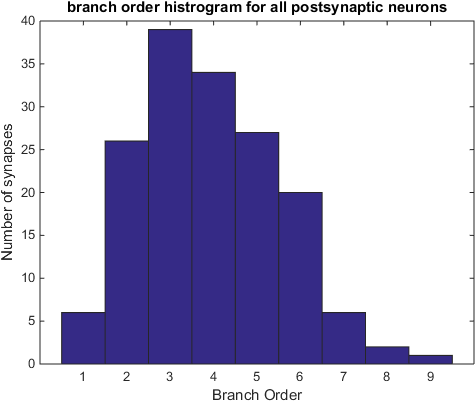
Histogram with the postsynaptic branch orders of all synapses.
disp('Calculating Projections') ;
%Target density projections
YprojPre = densityProjection(lpar,Ypre,true) ;
% YprojPost = densityProjection(lpar,Ypre,true) ;

%synaptic element projections
XprojPre = densityProjection(lpar,Xpre) ;
% XprojPost = densityProjection(lpar,Xpost) ;

% Calculating soma projections
%Soma projection resolution (in voxels)
SomaDensResolution = 5 ;
%Soma density projections, SomaDensResolution is defined above
somDensPre = somaDens3D(lpar,Yinfo(lpar.preIndex),SomaDensResolution) ;
somDensPost = somaDens3D(lpar,Yinfo(lpar.postIndex),SomaDensResolution) ;
%Special one, synaptic element projectiosn, yse genSynX to generate a
%matrix of X's shape from the synNeurMap
synProjPre = densityProjection(lpar,genSynX(lpar,synNeurMap,[],[],true)) ;
%Showing the connectivity matrix
figure(2)
showConMat(conMat,CMmsrs) ;
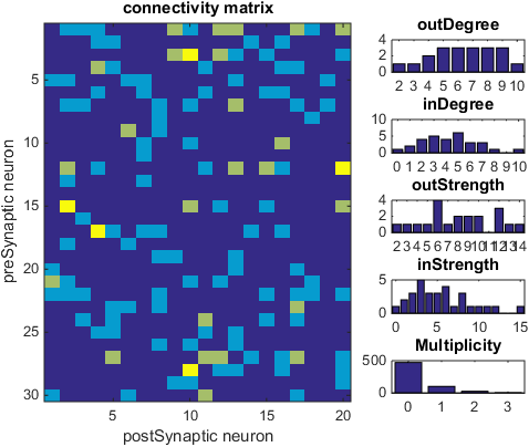
Connectivity matrix and associated measures. Each square has a color based on the number of synapses between the associated two neurons. The Degree is the number of connected neurons, and the strength is the total number of synapses. In and out correspond to the postsynaptic and presynaptic population respecitively. The multiplicity is the number of synapses between any two neurons, consequently the last histogram is a histogram over all the colors of the squares.
%Showing Projections
figure(3) ;
showProjections(lpar,YprojPre,XprojPre,synProjPre) ;
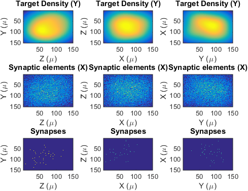
Projections (not slices) of the target density, the genereated synaptic elements and the generated synapses of the presynaptic population.
figure(4);
showProjections(lpar,Ypost,Xpost)
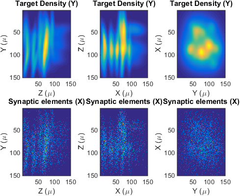
Projections (not slices) of the target density, the genereated synaptic elements of the postsynaptic population.
%Showing soma density projections
figure(5)
subplot(1,3,1) ;
imagesc(somDensPre.X);
xlabel('Z (bins)');
ylabel('Y (bins)');
title('Soma') ;
subplot(1,3,2) ;
imagesc(somDensPre.Y);
xlabel('X (bins)');
ylabel('Z (bins)');
title('Soma') ;
subplot(1,3,3) ;
imagesc(somDensPre.Z);
xlabel('Y (bins)');
ylabel('X (bins)');
title('Soma') ;
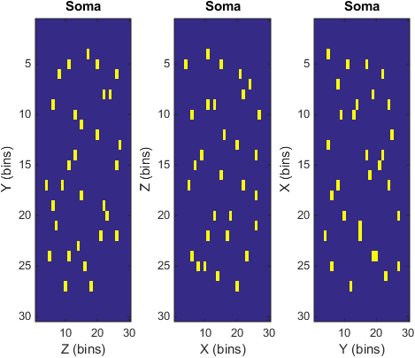
Projected soma locations
% RecenterPlot
figure(6)
recenterPlot(lpar,Xpost,Yinfo{lpar.postIndex}) ;
title('Synaptic elements of all postsynaptic neurons, relative to soma and unrotated') ;
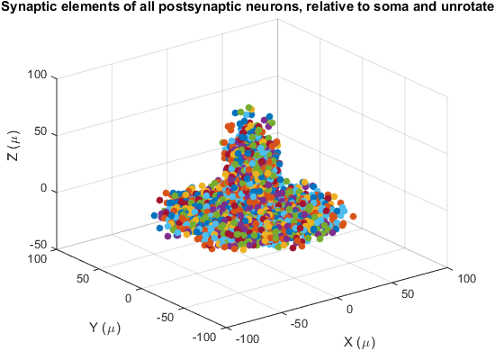
Recenterplot shows the synaptic elements of one population. Unlike showY, the synaptic elements are not plotted by their location in world coordinates, but relative to the soma, with the axes of the generator aligned.
The following sections uses several plotting functions starting with show, namely, showY, showSoma,showTrees and showSynapses. It is left as an excersize for the reader to figure out what their function is. Another function that belongs to this list is showX. For More information see the respective help files.
%for what neurons do we show everything
whichNeuronExtensively = [2 8] ;

figure(7);clf
%soma plot color
somaColor = [0 0 1] ;

showY(lpar,Ypost(:,whichNeuronExtensively)) ;
hold on ;
%show alls soma
showSoma(lpar,Yinfo,false,[],somaColor,'.')
%Plotting functions clear the axes if hold is off
%show some trees
showTrees(TreesPost(whichNeuronExtensively),[],'-p')
axis equal
%Synapse colormap
otherCc= [1 1 1; somaColor;distinguishable_colors(numel(whichNeuronExtensively))];
synapseCC = distinguishable_colors(lpar.postN,otherCc) ;
%add the synapses
showSynapses(lpar,synNeurMap,[],whichNeuronExtensively,true,synapseCC) ;
Two neurons in their full glory; Soma, Target density, generated tree (where each corner is a generated synaptic element), and synapses. The synapse colors represent different presynaptic partners.