
This is a more realistic model of thalamocortical projections to L4 spiny stellate cells. Thalamocortical projection axon denisties are again modelled as quasi randomly distributed spherical Gaussians. Spiny Stellate cell densities on the other hand are now derived from real data, by taking six reconstructed spiny stellate cells and fitting a 14-component Gaussian mixture model to each of them. Two versions of this Two versions of this model are used as examples. This version limits the number of postsynaptic neurons and the number of voxels to be able to generatea whole neuron in a whole barrel. The other version@@link@@ uses all realistic values, but only generates a part of the barrel.
References:
[1] Dimensions of a projection column and architecture of VPM and POm axons in rat vibrissal cortex. Wimmer VC, Bruno RM, de Kock CP, Kuner T, Sakmann B. Cereb Cortex. 2010 Oct;20(10):2265-76 [2] Number and laminar distribution of neurons in a thalamocortical projection column of rat vibrissal cortex. Meyer HS, Wimmer VC, Oberlaender M, de Kock CP, Sakmann B, Helmstaedter M. Cereb Cortex. 2010 Oct;20(10):2277-86 [3] Cell type-specific thalamic innervation in a column of rat vibrissal cortex. Meyer HS, Wimmer VC, Hemberger M, Bruno RM, de Kock CP, Frick A, Sakmann B, Helmstaedter M. Cereb Cortex. 2010 Oct;20(10):2287-303 [4] Functional diversity of layer IV spiny neurons in rat somatosensory cortex: quantitative morphology of electrophysiologically characterized and biocytin labeled cells. Staiger JF, Flagmeyer I, Schubert D, Zilles K, Koetter R, Luhmann HJ.Cereb Cortex. 2004 Jun;14(6):690-701
clear lpar
lpar.nDim = 3;
lpar.nSigRange = 2 ;

lpar.vox.voxelSize = 3; %voxel size is set to three micron
lpar.vox.voxPerDim = ceil([370 370 263]./lpar.vox.voxelSize) ; %L4 of one barrel is about this size [2] (in number of voxels)

%definition of a neural population
%Seed for this population
postPop.seed = 27552 ;
postPop.name = 'Spiny Stellate Dendrites' ;
postPop.nr = 1 ;
postPop.isPre = 0 ;

postPop.Nn = 10 ;
postPop.soma.edge = 0.3 ;
postPop.soma.distr = 'qrand' ;
postPop.soma.seed = 2421 ;

%Set the typeSpec from fitted neurons. This also requires changing Yinfo
%after prepareForYgen. (see below). The mat file can be generated from
%neuron reconstructions using the trees toolbox to load and resample them,
%and MATLABS gmdistribution.fit to generate the fit.
[postPop.typeSpec, wVecC]= loadTypeSpecFromMatFile('GMfit_BlueBrain_MB') ;
%make sure to use all neurons, for more information see 'help randSample'
postPop.typeSpec.neuronNumberDistr = 'alli' ;

%Trees balancing factor
postPop.mst.bf = [.55 0.025] ;
postPop.mst.bfDistr = 'normal' ;
%Trees max branch threshold
postPop.mst.thr = [100] ;

lpar.neurPop{1} = postPop ;
% define second population
prePop.isPre = 1 ;
prePop.Nn = 50 ; %Actual number not available
prePop.seed = 18713 ;
prePop.name = 'VPM projection neurons' ; %[1] ventral postmedial axons project to the barrels
prePop.soma.edge = 0.1 ;
prePop.soma.distr = 'qrand' ; %quasi random, like random, but more uniform
prePop.soma.seed = 294312;

prePop.typeSpec.generator = @(x) genGauss(x);
prePop.typeSpec.sig = [20 40] ;

%Trees balancing factor
prePop.mst.bf = [0.55 0.025] ;
prePop.mst.bfDistr = 'normal' ;
%Trees max branch threshold
prePop.mst.thr = [100] ;

lpar.neurPop{2} = prePop ;

[lpar,Yinfo] = prepareForYgen(lpar) ;
% Because of the design of the program, the weight vector from fits should be set after prepareForYgen
newWvec = arrayfun(@(x) wVecC{1}{x},Yinfo{1}.sampled.typeSpec.neuronNumber,'uni',0);
Yinfo{1}.sampled.typeSpec.wVec = cell2mat(newWvec);
[lpar,Yinfo] = preparePartialY(lpar,Yinfo) ;
[Ypre,Ypost] = generateY(lpar,Yinfo) ;
nSynPreMean = 1000 ;
nSynPreSig = 300 ;
nSynPostMean = 300 ;
nSynPostSig = 70 ;
removeOverlap = true ;
TreeJitterAmplitude = 1 ;

disp('Generating presynaptic elements') ;
[Xpre] = genRand1(Ypre,nSynPreMean,nSynPreSig,removeOverlap) ;
disp('Generating postsynaptic elements') ;
[Xpost] = genRand1(Ypost,nSynPostMean,nSynPostSig,removeOverlap) ;
disp('Generating presynaptic trees') ;

[ TreesPre,synBOpre ] = growTrees(lpar,Xpre,Yinfo,true,TreeJitterAmplitude) ;
disp('Generating postsynaptic trees') ;
[ TreesPost,synBOpost ] = growTrees(lpar,Xpost,Yinfo,false,TreeJitterAmplitude) ;
disp('Generating Connectivity matrix') ;
[conMat,synNeurMap] = generateConnectivity(Xpre,Xpost) ;
disp('Calculating measures') ;
figure(1)
Ymsrs = Ymeasures(Ypre,Ypost,true) ;
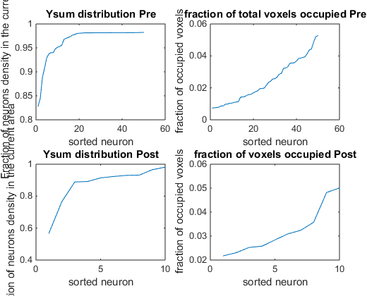
Selected Y measures. These graphs quickly show wether the generated neurons have a significant portion of their density in the generated part of the world.
XmsrsPre = Xmeasures(lpar,Xpre)
XmsrsPost = Xmeasures(lpar,Xpost)

disp('Calculating Projections') ;
XprojPre = densityProjection(lpar,Xpre) ;
XprojPost = densityProjection(lpar,Xpost) ;
YprojPre = densityProjection(lpar,Ypre,true) ;
YprojPost = densityProjection(lpar,Ypost,true) ;

disp('Calculating branch order distributions') ;
boSynListPre = branchOrderDistr(synBOpre,synNeurMap,true) ;
boSynListPost = branchOrderDistr(synBOpost,synNeurMap,false) ;
%use pipelinePlot to generate some of the figures from the manual
% pipelinePlot(lpar,Ypost,Xpost,TreesPost,1:4:5,1,5)

figure(2)
hist(cell2mat(boSynListPost)) ;
title('Branch order histrogram, for all postsynaptic neurons');
xlabel('Branch Order') ;
ylabel('Number of synapses') ;
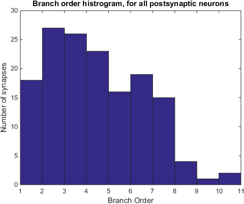
Histogram with the branch orders of all synapses.
figure(3)
showConMat(conMat)
title('Connectivity matrix');
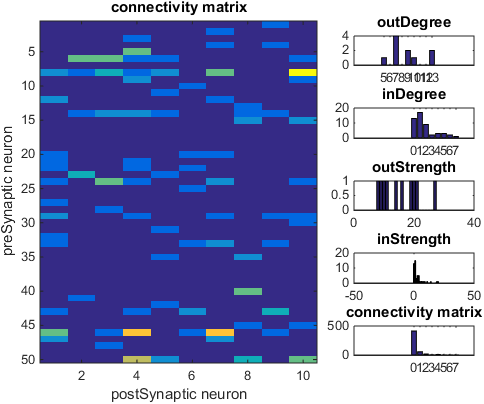
Connectivity matrix and associated measures. Each square has a color based on the number of synapses between the associated two neurons. The Degree is the number of connected neurons, and the strength is the total number of synapses. In and out correspond to the postsynaptic and presynaptic population respecitively. The multiplicity is the number of synapses between any two neurons, consequently the last histogram is a histogram over all the colors of the squares.
figure(4)
somaColor = [1 0 0] ;
treeColor = [1 0 0] ;
densColor = [1 0 0] ;
%Somasizes depend on number of synaptic elements
somaSizeArr = (XmsrsPost.nSynElArr / max(XmsrsPost.nSynElArr(:))).^2 * 4;
showSoma(lpar,Yinfo,false,somaSizeArr,somaColor)

hold on ;
whichNeuron = 4 ;
showY(lpar,Ypost(:,whichNeuron),densColor)
axis equal
showTrees(TreesPost(whichNeuron),treeColor,'-p')
synapseCC = distinguishable_colors(lpar.postN,[1 1 1; somaColor]) ;
showSynapses(lpar,synNeurMap,[],whichNeuron,true,synapseCC) ;
hold off
title('All soma, One target density, tree and associated synapses (colored by presynaptic neuron)');
setLimToWorld(lpar) ;
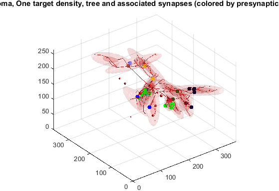
Here you see one neuron with everything related. See through are the isosurfaces of the target density (Y), the red branches is the generated neuron, the colored dots are the synapsesm with different colors for different partners, and the red spheres are the soma of the other postsynaptic neurons, where their somasize depends on the number of synaptic elements.